Specifying Accelerated Failure Time Models in STAN
This post is an add-on to my previous post about augmented gibbs sampling for censored survival times. If you’re not a complete maniac like me, then you probably don’t want to code your own sampler from scratch like I did in that previous post. Luckily you don’t have to because you can easily specify that same model in Stan.
Let’s start with simulating some randomly censored data from a Weibull model. In this case, we just include a binary indicator and are interested in characterizing survival between these two groups.
set.seed(1)

n <- 1000

# simulate covariates (just a binary treatment indicator)
A <- rbinom(n, 1, .5)
X <- model.matrix(~ A)

# true parameters
true_beta <- (1/2)*matrix(c(-1/3, 2), ncol=1)
true_mu <- X %*% true_beta

true_sigma <- 1

true_alpha <- 1/true_sigma
true_lambda <- exp(-1*true_mu*true_alpha)

# simulate censoring and survival times
survt = rweibull(n, shape=true_alpha, scale = true_lambda)
cent = rweibull(n, shape=true_alpha, scale = true_lambda)

## observed data:
#censoring indicator
delta <- cent < survt
survt[delta==1] <- cent[delta==1] # censor survival time.

# count number of missing/censored survival times
n_miss <- sum(delta)

d_list <- list(N_m = n_miss, N_o = n - n_miss, P=2, # number of betas
               # data for censored subjects
               y_m=survt[delta==1], X_m=X[delta==1,],
               # data for uncensored subjects
               y_o=survt[delta==0], X_o=X[delta==0,])
The list d_list is what we’ll eventually feed to Stan. Below is the Stan model for Weibull distributed survival times. Note in the transformed parameters block we specify the canonical accelerated failure time (AFT) parameterization - modeling the scale as a function of the shape parameter, \(\alpha\), and covariates.
In the model block, we specify the likelihood as the Weibull density for uncensored subjects, and then augment the likelihood with evaluations from the Weibull survival function (_lccdf).
The generated quantities block transforms the parameters to get posterior draws of the hazard ratio (as specified in my previous post ) as well as posterior draws of the survival function.
data {
  int<lower=0> P; // number of beta parameters

  // data for censored subjects
  int<lower=0> N_m;
  matrix[N_m,P] X_m;
  vector[N_m] y_m;

  // data for observed subjects
  int<lower=0> N_o;
  matrix[N_o,P] X_o;
  real y_o[N_o];
}

parameters {
  vector[P] beta;
  real<lower=0> alpha; // Weibull Shape
}

transformed parameters{
  // model Weibull rate as function of covariates
  vector[N_m] lambda_m;
  vector[N_o] lambda_o;

  // standard weibull AFT re-parameterization
  lambda_m = exp((X_m*beta)*alpha);
  lambda_o = exp((X_o*beta)*alpha);
}

model {
  beta ~ normal(0, 100);
  alpha ~ exponential(1);

  // evaluate likelihood for censored and uncensored subjects
  target += weibull_lpdf(y_o | alpha, lambda_o);
  target += weibull_lccdf(y_m | alpha, lambda_m);
}


// generate posterior quantities of interest
generated quantities{
  vector[1000] post_pred_trt;
  vector[1000] post_pred_pbo;
  real lambda_trt;
  real lambda_pbo;
  real hazard_ratio;

  // generate hazard ratio
  lambda_trt = exp((beta[1] + beta[2])*alpha ) ;
  lambda_pbo = exp((beta[1])*alpha ) ;

  hazard_ratio = exp(beta[2]*alpha ) ;

  // generate survival times (for plotting survival curves)
  for(i in 1:1000){
    post_pred_trt[i] = weibull_rng(alpha,  lambda_trt);
    post_pred_pbo[i] = weibull_rng(alpha,  lambda_pbo);
  }
}
The Stan model specified above is stored in an object called weibull_mod, which is called below in sampling(). The code below samples from the posterior and outputs posterior draws of the hazard and predicted survival times.
weibull_fit <- sampling(weibull_mod,
                data = d_list,
                chains = 1, iter=20000, warmup=19000, save_warmup=F,
                pars= c('hazard_ratio','post_pred_trt','post_pred_pbo'))
##
## SAMPLING FOR MODEL '80acc0f9293b946800a710dd7f5e211c' NOW (CHAIN 1).
## Chain 1:
## Chain 1: Gradient evaluation took 0.000172 seconds
## Chain 1: 1000 transitions using 10 leapfrog steps per transition would take 1.72 seconds.
## Chain 1: Adjust your expectations accordingly!
## Chain 1:
## Chain 1:
## Chain 1: Iteration: 1 / 20000 [ 0%] (Warmup)
## Chain 1: Iteration: 2000 / 20000 [ 10%] (Warmup)
## Chain 1: Iteration: 4000 / 20000 [ 20%] (Warmup)
## Chain 1: Iteration: 6000 / 20000 [ 30%] (Warmup)
## Chain 1: Iteration: 8000 / 20000 [ 40%] (Warmup)
## Chain 1: Iteration: 10000 / 20000 [ 50%] (Warmup)
## Chain 1: Iteration: 12000 / 20000 [ 60%] (Warmup)
## Chain 1: Iteration: 14000 / 20000 [ 70%] (Warmup)
## Chain 1: Iteration: 16000 / 20000 [ 80%] (Warmup)
## Chain 1: Iteration: 18000 / 20000 [ 90%] (Warmup)
## Chain 1: Iteration: 19001 / 20000 [ 95%] (Sampling)
## Chain 1: Iteration: 20000 / 20000 [100%] (Sampling)
## Chain 1:
## Chain 1: Elapsed Time: 12.2212 seconds (Warm-up)
## Chain 1: 1.03363 seconds (Sampling)
## Chain 1: 13.2548 seconds (Total)
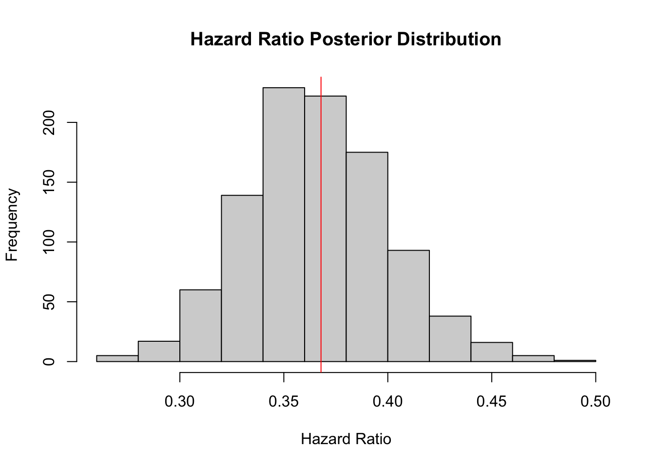
## Chain 1:post_draws<-extract(weibull_fit)Below we plot posterior distribution of the hazard ratio. The red line indicates the true value under which we generated the data.
hist(post_draws$hazard_ratio,
     xlab='Hazard Ratio', main='Hazard Ratio Posterior Distribution')
abline(v=exp(-1*true_beta[2,1]*true_alpha), col='red')
mean(post_draws$hazard_ratio)## [1] 0.3658342quantile(post_draws$hazard_ratio, probs = c(.025, .975))## 2.5% 97.5%
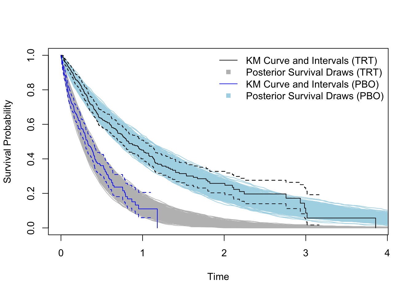
## 0.3039049 0.4376196Below we plot the survival functions. Note these results are very similar to the augmented sampler coded in the previous post.
plot(survfit(Surv(survt, 1-delta) ~ A ), col=c('black','blue'),
     xlab='Time',ylab='Survival Probability', conf.int=T)

for(i in 1:1000){
  trt_ecdf <- ecdf(post_draws$post_pred_trt[i,])
  curve(1 - trt_ecdf(x), from = 0, to=4, add=T, col='gray')

  pbo_ecdf <- ecdf(post_draws$post_pred_pbo[i,])
  curve(1 - pbo_ecdf(x), from = 0, to=4, add=T, col='lightblue')
}

lines(survfit(Surv(survt, 1-delta) ~ A ), col=c('black','blue'), add=T,
      conf.int=T)

legend('topright',
       legend = c('KM Curve and Intervals (TRT)',
                  'Posterior Survival Draws (TRT)',
                  'KM Curve and Intervals (PBO)',
                  'Posterior Survival Draws (PBO)'),
       col=c('black','gray','blue','lightblue'),
       lty=c(1,0,1,0), pch=c(NA,15,NA,15), bty='n')