Bayesian Survival Analysis with Data Augmentation

Motivation

When dealing with time-to-event data, right-censoring is a common occurance. Although most are familiar with likelihood construction under right-censoring (and corresponding frequentist estimation), there’s very little available online about Bayesian approaches even for fully parametric models. Here I’ll briefly outline a Bayesian estimation procedure for a Weibull model with right-censoring. The estimation procedure is MCMC based using a data augmentation approach.

As with most of my posts, all MCMC is coded from scratch. It helps me and it helps readers understand the underlying algorithm - an intuition that is more difficult to get if you’re just specifying the model in Stan.

Model Set Up

Suppose we observe $i=1,\dots ,r$ survival times, $T_i^o$. Survival times past the end of our study (at time $\tau$) are censored for subjects $i=r+1,\dots ,n$. We know that the survival times for these subjects are greater than $\tau$, but that is all. Say we also have some $p\times 1$ covariate vector, $x_i$. Finally, we have indicator of whether survival time is observed ${\delta }_{1:n}$ for each subject. A parametric approach follows by assuming a model for $T$, we choose the Weibull

$$T_i^o\sim Weibull(\alpha ,{\lambda }_i)$$ Where $\alpha$ is the shape parameter and ${\lambda }_i$ is a subject-specific scale. An Accelerated Failure Time model (AFT) follows from modeling a reparameterization of the scale function ${\lambda }_i=exp(-{\mu }_i\alpha )$, where ${\mu }_i=x_i^T\beta$.

We’ll consider the setting where we regress on a binary treatment indicator, ${\mu }_i={\beta }_0+{\beta }_{1}A$ where $A=1$ indicates treated and $A=0$ indicates untreated/placebo. This is a funky reparameterization, but it yields intuitive interpretations for ${\beta }_1$ in terms of the Weibull’s hazard function, $h(t|\beta ,x,\alpha )={\lambda }_i\alpha x^{\alpha -1}$. Substituting ${\lambda }_i$, we see the hazard for treated subjects is $h(t|A=1)=e^{-({\beta }_0+{\beta }_1)\ast \alpha }\alpha t^{\alpha -1}$ and for untreated subjects it is $h(t|A=1)=e^{-({\beta }_0)\ast \alpha }\alpha t^{\alpha -1}$. The hazard ratio is,

$$HR=\frac{h(t|A=1)}{h(t|A=0)}=e^{-{\beta }_1\ast \alpha }$$ If $HR=.5$, then the hazard of death, for example, at time $t$ is $50\mathrm{\%}$ lower in the treated group, relative to the untreated.

From a Bayesian point of view, we are interested in the posterior $p(\beta ,\alpha |T_{1:r}^o,{\delta }_{1:n},\tau )$. Once we have this, we can get a whole posterior distribution for the survival function itself - as well as any quantity derived from it. For example, posterior mean and credible intervals for $HR$ (just a function of ${\beta }_1$ and $\alpha$). We can also get posterior survival curve estimates for each treatment group. For the Weibull, the survival curve is given by $S(t|\beta ,\alpha ,A)=exp(-\lambda t^{\alpha })$ - again just a function of ${\beta }_1$ and $\alpha$.

Data Augmentation

We’ll first look at the joint data distribution (the likelihood) for this problem. The central idea is to view the survival times for the $n-r$ censored subjects as missing data, $T_{r+1:n}^m$. We refer to the full data as $T_{i=1:n}=(T_{i:r}^o,T_{r+1:n}^m)$. Now we construct a complete-data (augmented) likelihood with these values. The observed likelihood and complete-data likelihood are related by

$$\begin{array}{rl}p(T_{1:r}^o,{\delta }_{1:n}|\tau ,\beta ,\alpha )& =\int p(T_{1:n},{\delta }_{1:n}|\tau ,\beta ,\alpha )d{T}_{r+1:n}^m\\ & =\int p({\delta }_{1:n}|T_{1:n},\tau ,\beta ,\alpha )p(T_{1:n}|\tau ,\beta ,\alpha )d{T}_{r+1:n}^m\end{array}$$ Now in this ideal, complete-data setting, we observe patients with either ${\delta }_i=1\cap T_i>\tau$ or with ${\delta }_i=0\cap T_i<\tau$. That is, $p({\delta }_i|T_i,\tau ,\beta ,\alpha )=1$ if either of these conditions hold and $0$ otherwise.

We also assume that subjects are independent so that $p(T_{i=1:n}|\tau ,\beta ,\alpha )=p(T_{1:r}^o|\tau ,\beta ,\alpha )p(T_{r+1:n}^m|\tau ,\beta ,\alpha )$. So the likelihood simplifies to: $$\begin{array}{rl}p(T_{1:r}^o,{\delta }_{1:n}|\tau ,\beta ,\alpha )& =\prod _{i=1}^n\int p({\delta }_i|T_i,\tau ,\beta ,\alpha )p(T_i|\tau ,\beta ,\alpha )d{T}_{r+1:n}^m\\ & =\prod _{i|{\delta }_i=0}p(T_i^o|\tau ,\beta ,\alpha )\prod _{i|{\delta }_i=1}\int p({\delta }_i|T_i^m,\tau ,\beta ,\alpha )p(T_i^m|\tau ,\beta ,\alpha )d{T}_i^m\\ & =\prod _{i|{\delta }_i=0}p(T_i^o|\tau ,\beta ,\alpha )\prod _{i|{\delta }_i=1}\int I(T_i^m>\tau )p(T_i^m|\tau ,\beta ,\alpha )d{T}_i^m\\ & =\prod _{i|{\delta }_i=0}p(T_i^o|\tau ,\beta ,\alpha )\prod _{i|{\delta }_i=1}{\int }_{\tau }^{\mathrm{\infty }}p(T_i^m|\tau ,\beta ,\alpha )d{T}_i^m\end{array}$$ The first line follows by independence of observations. The second line follows by separating censored and uncensored subjects. $p({\delta }_i|-)=1$ for all uncensored subjects, but $p({\delta }_i|-)=1$ for censored subjects only when $T_i^m\in (0,\mathrm{\infty })$. Otherwise, the integrand is 0. Therefore, in the fourth line we only need to integrate of the region where the integrand is non-zero.

Now the integral is over the region $T_i^m\in (0,\mathrm{\infty })$. But in this region $p({\delta }_i|T_i^m,\tau ,\beta ,\alpha )=1$ only when $T_i^m>\tau$.

This is the usual likelihood for frequentist survival models: uncensored subjects contribute to the likelihood via the density while censored subjects contribute to the likelihood via the survival function ${\int }_{\tau }^{\mathrm{\infty }}p(T_i^m|\tau ,\beta ,\alpha )d{T}_i^m$. Functions for this integral exist in for most basic distributions in R. For our Weibull model, it is 1-pweibull(). We would simply place priors on $\beta$ and $\alpha$, then sample from the posterior using MCMC.

But what if this integral was too hard to evaluate (as it may be for more complicated censoring mechanisms) and the complete data likelihood given below is easier?

$$\begin{array}{rl}p(T_{1:r}^o,T_{r+1:n}^m,{\delta }_{1:n}|\tau ,\beta ,\alpha )& =\prod _{i|{\delta }_i=0}p(T_i^o|\tau ,\beta ,\alpha )\prod _{i|{\delta }_i=1}I(T_i^m>\tau )p(T_i^m|\tau ,\beta ,\alpha )\end{array}$$ Then we can design a Gibbs sampler around this complete data likelihood.

Metropolis-in-Gibbs Sampler

The target posterior of interest is $$p(\beta ,\alpha ,T_{r+1:n}^m|T_{1:r}^o,{\delta }_{1:n})=p(\beta ,\alpha |T_{r+1:n}^m,T_{1:r}^o,{\delta }_{1:n})p(T_{r+1:n}^m|\beta ,\alpha ,T_{1:r}^o,{\delta }_{1:n})$$ Where each conditional posterior is known up to a proportionality constant. With a joint prior $p(\beta ,\alpha )$ specified, we have

$$\begin{array}{rl}p(\beta ,\alpha |T_{r+1:n}^m,T_{1:r}^o,{\delta }_{1:n})& \propto \prod _{i|{\delta }_i=0}p(T_i^o|\tau ,\beta ,\alpha )\prod _{i|{\delta }_i=1}I(T_i^m>\tau )p(T_i^m|\tau ,\beta ,\alpha )\\ & \propto p(\beta ,\alpha )\prod _{i=1}^{n}p(T_i|\tau ,\beta ,\alpha )\end{array}$$ Note here that $p(T_i|\tau ,\beta ,\alpha )$ is the assumed Weibull density. We can use a Metropolis step to sample $(\beta ,\alpha )$ from this distribution.

The second conditional posterior is $$\begin{array}{r}p(T_{r+1:n}^m|\beta ,\alpha ,T_{1:r}^o,{\delta }_{1:n})\propto \prod _{i|{\delta }_i=1}I(T_i^m>\tau )p(T_i^m|\tau ,\beta ,\alpha )\end{array}$$ This is a truncated Weibull distribution (truncated at the bottom by $\tau$). We can also sample from this using a Metropolis step.

The Gibbs sampler alternates between sampling from these two conditionals:

1. Given parameters $(\beta ,\alpha )$, impute $T_i^m$ by drawing from $p(T_{r+1:n}^m|\beta ,\alpha ,T_{1:r}^o,{\delta }_{1:n})$, for each $i=r+1,\dots ,n$.
2. Combine these imputed values, $T_{r+1:n}^m$, with observed data $T_{1:n}^o$, and update the parameters $(\beta ,\alpha )$ from $p(\beta ,\alpha |T_{r+1:n}^m,T_{1:r}^o,{\delta }_{1:n})$.

As the parameter estimates update, the imputations get better. As the imputations get better, the parameter estimates improve. Over time the process yields draws from the joint posterior $p(\beta ,\alpha ,T_{r+1:n}^m|T_{1:r}^o,{\delta }_{1:n})$

We retain the sample of $(\beta ,\alpha )$ for inference and toss samples of $T^m$.

Simulation Example in R

All of the code implementing the augmented sampler (from scratch!) can be found on my GitHub. Basically I simulate a data set with a binary treatment indicator for 1,000 subjects with censoring and survival times independently drawn from a Weibull. \

For the $\beta$ vector, I use independent $N(0,sd=100)$ priors. For the shape parameter, I use an $Exp(1)$ prior. I run a single MCMC chain for 20,000 iterations and toss the first 15,000 out as burn-in.

Here is the estimated survival function for each treatment group. Overlayed are the non-parametric estimates from a stratified Kaplan-Meier (KM) estimator. Note the parametric model is correctly specified here, so it does just as well as the KM in terms of estimating the mean curve. But the parametric model provides a less noisy fit - notice the credible bands are narrower at later time points when the at-risk counts get low in each treatment arm.

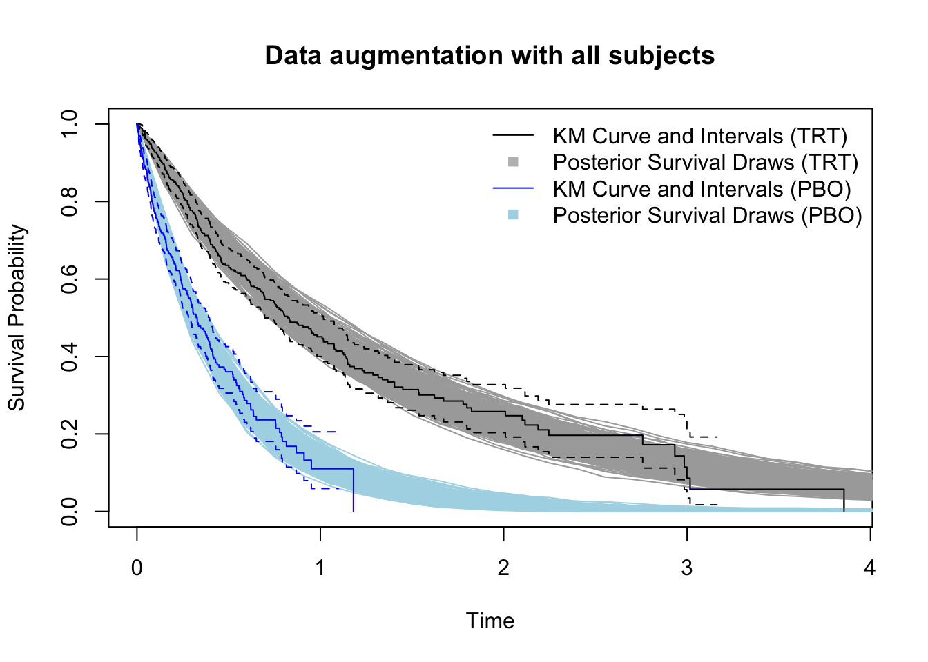
That’s just a helpful reminder of the efficiency gains parametric models have over nonparametric ones (when they’re correctly specified. Let’s take a look at the posterior distribution of the hazard ratio. The true value is indicated by the red line.

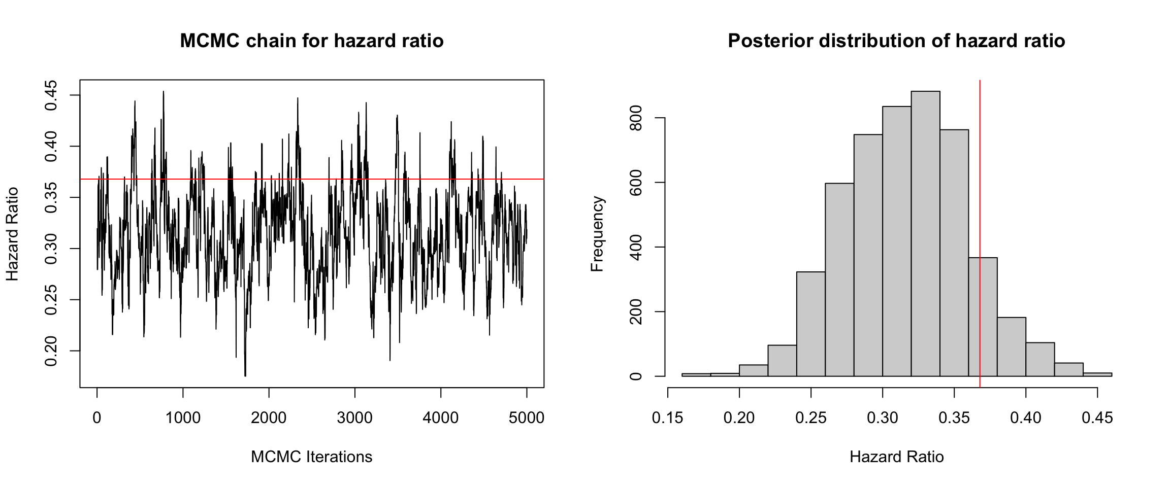We could have run this thing for longer (and with multiple chains with different starting values). But I think this gets the point across. The posterior mean and $95\mathrm{\%}$ credible interval are $.32(.24-.40)$. The true value is $.367$. Not too bad. Remember this is only a single simulated dataset.