Gamma Process Prior for Semiparametric Survival Analysis
Heads up: equations may not render on blog aggregation sites. See original post here for good formatting. If you like this post, you can follow me on twitter.
Motviation
Suppose we observe survival/event times from some distribution \[T_{i\in1:n} \stackrel{iid}{\sim} f(t)\] where \(f\) is the density and \(F(t)=1-S(t)\) is the corresponding CDF expressed in terms of the survival function \(S(t)\). We can represent the hazard function of this distribution in terms of the density, \[\lambda(t) = \frac{f(t)}{S(t)}\] The hazard, CDF, and survival functions are all related. Thus, if we have a model for the hazard, we also have a model for the survival function and the survival time distribution. The well-known Cox proportional hazard approach models the hazard as a function of covariates \(x_i \in \mathbb{R}^p\) that multiply some baseline hazard \(\lambda_0(t)\), \[ \lambda(t_i) = \lambda_0(t_i)\exp(x_i'\theta)\] Frequentist estimation of \(\theta\) follows from maximizing the profile likelihood - which avoids the need to specify the baseline hazard \(\lambda_0(t)\). The model is semi-parametric because, while we don’t model the baseline hazard, we require that the multiplicative relationship between covariates and the hazard is correct.
This already works fine, so why go Bayesian? Here are just a few (hopefully) compelling reasons:
- We may want to nonparametrically estimate the baseline hazard itself.
- Posterior inference is exact, so we don’t need to rely on asymptotic uncertainty estimates (though we may want to evaluate the frequentist properties of resulting point and interval estimates).
- Easy credible interval estimation for any function of the parameters. If we have posterior samples for the hazard, we also get automatic inference for the survival function as well.
Full Bayesian inference requires a proper probability model for both \(\theta\) and \(\lambda_0\). This post walks through a Bayesian approach that places a nonparametric prior on \(\lambda_0\) - specifically the Gamma Process.
The Gamma Process Prior
Independent Hazards
Most of this comes from Kalbfleisch (1978), with an excellent technical outline by Ibrahim (2001).
Recall that the cumulative baseline hazard \(H_0(t) = \int_0^t \lambda_0(t) dt\) where the integral is the Riemann-Stieltjes integral. The central idea is to develop a prior for the cumulative hazard \(H_0(t)\), which will then admit a prior for the hazard, \(\lambda_0(t)\).
The Gamma Process is such a prior. Each realization of a Gamma Process is a cumulative hazard function that is centered around some prior cumulative hazard function, \(H^*\), with a sort of dispersion/concentration parameter, \(\beta\) that controls how tightly the realizations are distributed around the prior \(H^*\).
Okay, now the math. Let \(\mathcal{G}(\alpha, \beta)\) denote the Gamma distribution with shape parameter \(\alpha\) and rate parameter \(\beta\). Let \(H^*(t)\) for \(t\geq 0\) be our prior cumulative hazard function. For example we could choose \(H^*\) to be the exponential cumulative hazard, \(H^*(t)= \eta\cdot t\), where \(\eta\) is a fixed hyperparameter. By definition \(H^*(0)=0\). The Gamma Process is defined as having the following properties:
- \(H_0(0) = 0\)
- \(\lambda_0(t) = H_0(t) - H_0(s) \sim \mathcal G \Big(\ \beta\big(H^*(t) - H^*(s)\big)\ , \ \beta \ \Big)\), for \(t>s\)
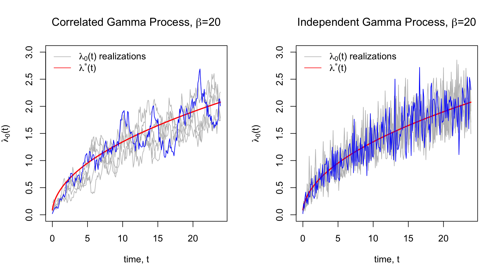
The increments in the cumulative hazard is the hazard function. The gamma process has the property that these increments are independent and Gamma-distributed. For a set of time increments \(t\geq0\), we can use the properties above to generate one realization of hazards \(\{\lambda_0(t) \}_{t\geq0}\). Equivaltently, one realization of the cumulative hazard function is \(\{H_0(t)\}_{t\geq0}\), where \(H_0(t) = \sum_{k=0}^t \lambda_0(k)\). We denote the Gamma Process just described as \[H_0(t) \sim \mathcal{GP}\Big(\ \beta H^*(t), \ \beta \Big), \ \ t\geq0\]
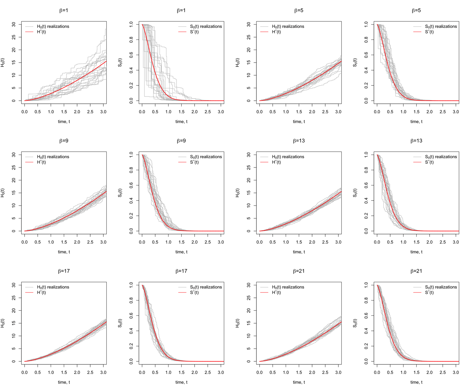
Below in Panel A are some prior realizations of \(H_0(t)\) with a Weibull \(H^*\) prior for various concentration parameters, \(\beta\). Notice for low \(\beta\) the realizations are widely dispersed around the mean cumulative hazard. Higher \(\beta\) yields to tighter dispersion around \(H^*\).
Since there’s a correspondence between the \(H_0(t)\), \(\lambda_0(t)\), and \(S_0(t)\), we could also plot prior realizations of the baseline survival function \(S_0(t) = \exp\big\{- H_0(t) \big\}\) using the realization \(\{H_0(t)\}_{t\geq0}\). This is shown in Panel B with the Weibull survival function \(S^*\) corresponding to \(H^*\).

